Author: samuel.cheng@ou.edu

Tulsa students now can directly apply for travel grants in Norman.

When the first president of the University of Oklahoma stepped off the train to look at his new environment, he exclaimed, “What possibilities!”    At the Gallogly College of Engineering, we’re still exploring what’s possible.   Join us! OU Engineering Information Session   Be part of the next generation of researchers   Join us to learn about: Graduate Programs Research and Opportunities Financial Support and Scholarships Alumni Engagement And more!   Monday, October 24, 2022 9:00am CDT   Zoom link will be provided upon registration.   Click Here to Register   For more information visit ou.edu/coe

Three Faculty Positions in Data Science: Human-Computer Teaming and  Interactive Decision Making; Artificial Intelligence Architectures; and Trustable  Artificial Intelligence at the University of Oklahoma, Norman Campus 

Positions Available: As part of a multiyear effort to grow world-class data science and data enabled research across The University of Oklahoma (OU), the Gallogly College of Engineering  (GCoE), Department of Electrical and Computer Engineering and/or Department of Computer  Science, in partnership with the Dodge Family College of Arts and Sciences (CAS), welcomes  applications for a cluster of three (3) faculty positions from candidates whose experiences and  interests have prepared them to be an integral contributor engaged in scientific discovery,  developing talent, solving global challenges, and serving our society. This year we are focusing  on data science foundational and enabling technologies. In subsequent years, we’ll be hiring  additional data science and data-enabled research faculty.  

The University, as part of its Lead On, University strategic plan has committed to creating world class capabilities in data science, artificial intelligence (AI), machine learning (ML), and data enabled research. In July 2020, the University established the Data Institute for Societal  Challenges (DISC) to grow convergent data-enabled research to solve global challenges. DISC  currently has over 130 faculty members across OU campuses, nine communities of practice, seed  funding programs, and an extended network of approximately 300 data scientists and data enabled researchers across many disciplines (https://www.ou.edu/disc). 

Three positions: 

1) Professor or Associate Professor in Human-Computer Teaming and Interactive  Decision Making: Humans and computers have complementary knowledge and skillsets.  To solve challenging problems, we need to team this expertise together for effectiveness,  reliability, efficiency, and adoption of many data-driven solutions. This area is cross 

disciplinary, and we seek a senior faculty member with expertise in one or more of human computer teaming, visualization, visual analytics, human-machine interaction, decision  theory, HCI, human factors and industrial engineering, or cognitive psychology. This  faculty member will be a vital core team member in data science and data-driven decision  making with a home department in ECE and possible joint appoint in ISE, Computer  Science, Psychology, and/or Political Science. 

Applications should be submitted online via Interfolio at  

http://apply.interfolio.com/112374. Inquires can be addressed to Professor David Ebert,  chair of the search committee at ebert@ou.edu.  

2) Assistant Professor in AI Architectures: We seek to recruit a transdisciplinary faculty  member with expertise in one or more of the following areas: scalable, high-performance  software and hardware architectures for AI and advanced analytics, advanced and  domain-tailored data science, AI (trustable, science-based, and human-guided), and  human-computer teaming. Specific areas of interest include probabilistic, neuromorphic,  and novel architectures, software pipelines and operating system architectures to support  high-performance analytics, and enable real-time trustable AI and decision-making.  Since  traditional computing architectures are still based on solving problems from the 20th  century, new computing hardware and software architectures are needed to optimize  computing for AI and machine learning and many new approaches to science and  engineering. This faculty member will grow and complement work in computer  engineering, computer science and the new OU quantum center (CQRT) with a home  department in ECE and possible joint appointments where appropriate.

Applications should be submitted online via Interfolio at   

http://apply.interfolio.com/112359.  Inquires can be addressed to Professor David Ebert,  chair of the search committee at ebert@ou.edu.  

3) Assistant Professor in Trustable AI. We are seeking an Assistant Professor in Trustable  AI. Human-guided, science-based, explainable AI (xAI) are key areas to ensure AI is  understandable, reliable, and robust for real-world applications. This faculty member will  grow our expertise in one of the most rapidly developing and vital fields of data science,  with a primary home in ECE and potentially joint appointments in CS, Psychology, and  ISE. We seek a faculty member with expertise in one or more of science-based AI or  machine learning (ML), human-guided AI/ML, explainable AI/ML, and closely related  topics.  This faculty member will be a vital core team member in data science, AI, and  data-driven convergent research solutions to global challenges. This faculty member will  provide vital capabilities that will empower research in all four strategic verticals and grow  the data science ecosystem on campus to create the critical mass in data science needed  for the success of the university’s strategic plan, Lead On, University. 

Applications should be submitted online via Interfolio at 

http://apply.interfolio.com/112372.  Inquires can be addressed to Professor David Ebert,  chair of the search committee at ebert@ou.edu.  

Gallogly College of Engineering:  The mission of the GCOE is to foster creativity, innovation and  professionalism through dynamic research, development and learning experiences.   

The Gallogly College of Engineering is home to the Data Science and Analytics Institute  (https://www.ou.edu/coe/dsai). The DSAI provides undergraduate and graduate certificates,  Master’s degrees, and PhD degrees in data science and analytics as well as offering workforce  upskilling to industry partners. Faculty members in GCoE and across campus participate in the  DSAI.  

The University of Oklahoma:  OU is a Carnegie-R1 comprehensive public research university  known for excellence in teaching, research, and community engagement, serving the educational,  cultural, economic and healthcare needs of the state, region, and nation from three campuses:  Norman, Health Sciences Center in Oklahoma City and the Schusterman Center in Tulsa. OU  enrolls over 30,000 students and has more than 2700 full-time faculty members in 21 colleges.   

Norman is a vibrant university town of around 113,000 inhabitants with a growing entertainment  and art scene. With outstanding schools, amenities, and a low cost of living, Norman is a perennial  contender on “best place to live” rankings.  

Visit http://www.ou.edu/flipbook and http://soonerway.ou.edu for more information. Within an easy  commute, Oklahoma City features a dynamic economy and outstanding cultural venues adding to  the region’s growing appeal.  

Qualifications 

Successful candidates must have the interest and ability to contribute significantly to the  advancement of these fields and develop a nationally recognized program of sponsored research;  teach at both the undergraduate and graduate levels; supervise graduate students and  postdoctoral fellows. A Ph.D. in computer science, engineering, or related discipline is required. 

Application Instructions 

Confidential review of applications will begin October 1, 2022. Candidates are invited to submit a 

letter of interest, names of three references who will be contacted only upon approval from the  applicant, curriculum vitae, and brief (~2-3 pages) statements of interest regarding 1) research, 2)  teaching, and 3) service. The research statement should summarize your prior contributions to  research and your goals for developing a research program at OU. The teaching statement should  summarize past instructional and mentorship experiences, and plans/goals for teaching at OU  (including existing and proposed courses) and advising a varied cohort of undergraduate and  graduate students. The service statement should describe your vision for internal service to the  academic unit, the College and the University, and for external service to our scientific community  and other stakeholders. Candidates are requested to submit their applications to the appropriate position listed above and inquiries should be directed to the search committee chairs, also listed  above. 

Inquiries should be directed to the search committee chair: 

Dr. David S. Ebert, Gallogly Chair Professor 

School of Electrical and Computer Engineering and School of Computer Science Associate Vice President of Research and Partnerships 

Director, Data institute for Societal Challenges  

University of Oklahoma 

Email: ebert@ou.edu 

Equal Employment Opportunity Statement  

The University of Oklahoma, in compliance with all applicable federal and state laws and  regulations does not discriminate on the basis of race, color, national origin, sex, sexual  orientation, genetic information, gender identity, gender expression, age, religion, disability,  political beliefs, or status as a veteran in any of its policies, practices, or procedures. This includes,  but is not limited to:  admissions, employment, financial aid, housing, services in educational  programs or activities, or health care services that the University operates or provides.  

Diversity Statement   

 The University of Oklahoma is committed to achieving a diverse, equitable and inclusive university  community by recognizing each person’s unique contributions, background, and perspectives. The  University of Oklahoma strives to cultivate a sense of belonging and emotional support for all,  recognizing that fostering an inclusive environment for all is vital in the pursuit of academic and  inclusive excellence in all aspects of our institutional mission.  

Mission of the University of Oklahoma 

The Mission of the University of Oklahoma is to provide the best possible educational  experience for our students through excellence in teaching, research and creative activity,  and service to the state and society.

I have a hard time standing manuscriptcentral. It is an absolute piece of crap. And unfortunately, it seems that the entire community is stuck with it. I am serving for AE for TCSVT this year. Like many journal publications, it was stuck with the crappy manuscriptcentral.

Just to be realistic, the hit rate of getting a reviewer is very low this day. I have created another tool to extract emails from hundreds of papers. I will now input close to 100 emails per manuscript to secure enough reviewers. It can take at least an hour to do that as manuscriptcentral do not have an import function. And the antiquated UI even expects an editor to input an email one by one.

So I tried to automate that using selenium. I am not an expert on that, but I saw another project using it and so tried to imitate what he did. It is part of the code below (after log in the page of the respective manuscript). And par is email extracted by my other tools. Basically, a csv file with the first two columns are the emails and names of the reviewers. The code is not very refined, but it did the trick.

from selenium.webdriver.common.by import By

for line in par.split('\n')[8:]:
    
    email=line.split(',')[0]
    firstname=line.split(',')[1].strip().split(' ')[0]
    lastname=line.split(',')[1].strip().split(' ')[1]    
    
    
    driver.switch_to.window(driver.window_handles[0])
    url='javascript:openCreateAccountPopup()'
    addReviewer = driver.find_element_by_xpath('//a[@href="'+url+'"]')
    addReviewer.click()


    driver.switch_to.window(driver.window_handles[1])
    # css_firstname = driver.find_element_by_css_selector('input[name="PERSON_FIRSTNAME"]')
    css_firstname=driver.find_element(By.NAME, "PERSON_FIRSTNAME")
    css_firstname.send_keys(firstname)
    css_lastname=driver.find_element(By.NAME, "PERSON_LASTNAME")
    css_lastname.send_keys(lastname)
    css_email=driver.find_element(By.NAME, "EMAIL_ADDRESS")
    css_email.send_keys(email)
    # css_firstname=driver.find_element(By.NAME, "XIK_ADD_FOUND_PERSON_ID")


    # add_reviewer_img = driver.find_element(By.src,"/images/en_US/buttons/create_add.gif")
    add_reviewer_img = driver.find_element(By.XPATH,"//img[@src='/images/en_US/buttons/create_add.gif']")

    add_reviewer_img.click()

    # case 1 (exist, save and add, best case)

    # add_reviewer_img = driver.find_element(By.src,"/images/en_US/buttons/create_add.gif")

    success=True
    try:
        add_reviewer_img = driver.find_element(By.XPATH,"//img[@src='/images/en_US/buttons/save_add.gif']")
        add_reviewer_img.click()
    except:
        success=False



    # case 2 (save and send email)

    # windows=driver.window_handles
    # print(windows)

    if not success:
        try:
            driver.switch_to.window(driver.window_handles[1])

            iframe = driver.find_element_by_name("bottombuttons")
            driver.switch_to.frame(iframe)


            # add_reviewer_img = driver.find_element(By.src,"/images/en_US/buttons/create_add.gif")
            add_save_send = driver.find_element(By.XPATH,"//img[@src='/images/en_US/buttons/save_send.gif']")

            add_save_send.click()
            success = True
        except:
            success = False

    # case 3 # select from existing, just pick one randomly


    if not success:
        try:
            add_save_send = driver.find_element(By.XPATH,"//img[@src='/images/en_US/buttons/add.gif']")
            add_save_send.click()
            success = True
        except:
            success = False

Below is a message from Ali Rhoades, an experiential learning coordinator.

For students interested in career readiness and job searches, I would encourage them to look into our events page including our Careerapalooza, Career Fair, and other events. Our Careerapalooza is coming up (next Thursday) but this would be a great opportunity for students to informally meet our staff, learn more about our support services (including applying for internship) and join a career community.

Our office just recently launched our Career Communities model, which encourages students to lean into finding internships and jobs specific to their passions and industry, instead of stressing to find experiential learning opportunities strict to their major. For example, if an engineering student was passionate for working in nonprofit, they would find tailored opportunities through their Nonprofit Career Community. This link will also provide them with access to their Handshake accounts (all OU students have free access to this internship and job board) including other helpful resources such as an advisor, additional job posting websites, and career readiness tips. Handshake will be the source where OU posts jobs, internships, externships, co-ops, and fellowships, which has new postings daily. If you would like one of our staff members to visit with your class to share more information about Career Communities and Handshake, please let me know-I’d be happy to set that up for you.

As for micro-internships: OU Career Center will be partnering with Parker Dewey soon, hopefully by the end of September, to have tailored micro-internships exclusively to OU students for local, remote, and regional opportunities that are short term and project based. Until then, students can look for public opportunities through Parker Dewey’s website here.

DDPG

Deep deterministic policy gradient (DDPG) is an actor-critic method. As the name suggests, the action is deterministic given the observation. DDPG composes of actor and critic networks. Given an observation, an actor network outputs an appropriate action. And given an action and an observation, a critic network outputs a prediction of the expected return (Q-value).

Replay Buffer

A replay buffer will store the (obs, action, reward, obs_next) tuples for each step the agent interacts with the environment. After the buffer is full, a batch of tuples can be extracted for training. Meanwhile, the new experience can be stored again in another buffer. Once the latter buffer is full, it can be swapped with the training buffer.

Training

A batch sampled from the replay buffer will be used to train the critic networks and then the actor networks. Then, another batch will be sampled and trained both networks again. As you will see, there are actually two critic and two actor networks in DDPG. The two networks in each type are almost identical but just one is a delayed or an average version of the other.

Training Actor Networks

We will fix the critic networks when we train the actor networks. Given a tuple (obs, action, reward, obs_next), we will only use the obs variable and plugged that into our actor network. The current actor network will create action_est and we can input both action_est and obs into the critic network to get an Q-value estimate. Assuming that the critic network is well-trained, the objective here is simply to maximize this estimated Q-value.

Training Critic Networks

Given a tuple (obs, action, reward, obs_next) and fixed actor networks, we have multiple ways to estimate an Q-value. For example, we can have

Q_est = critic_est (obs, action)

Q_tar = reward + discount critic_est (obs_next, act_est (obs_next))

The critic_est and act_est are critic and actor networks, respectively. So to train the network, we may try to minimize the square difference of Q_est and Q_tar.

Target Networks

As both Q_est and Q_tar depend on critic_est network, the naive implementation in training the critic networks tends to have poor convergence. To mitigate this problem, we can introduce a separate critic_est network. We will call this target critic network and denote it as critic_target. In practice, critic_target will simply be a delayed copy or an exponential average of critic_est. It seems that a target actor network, act_target, is introduced in the same manner. But I am not sure if it is really necessary.

TD3

TD3 stands for Twin Delayed DDPG. It is essentially DDPG but added with two additional tricks as follows.

Delayed Policy Update

The authors found that it is more important to have an accurate critic network than an actor network (similar to GAN that an accurate discriminator is important). Consequently, the authors suggest “delaying” the policy update. In practice, say train two batches of critic network before training a batch of actor network.

Clipped Double Q-Learning

Double Q-Learning was introduced to address the overestimation of Q-value. The authors argue that there is an overestimate of Q in DDPG as well. And they state that even double Q-learning is not sufficient to suppress the overestimation. Instead, they introduced a “clipped double Q-Learning”, where they use two critic networks rather than one to generate a current Q-estimate. And they aggregate the two estimates as the minimum of the two.

References:

• DDPG
• Addressing Function Approximation Error in Actor-Critic Methods (TD3)

Define policy and transition probability , the probability of a trajectory equal to

Denote the expected return as . Let’s try to find the improve a policy through gradient ascent by updating

Policy gradient and REINFORCE

Let’s compute the policy gradient ,

(1)  

With trajectories, we can approximate the gradient as

The resulting algorithm is known as REINFORCE.

Actor-critic algorithm

One great thing about the policy-gradient method is that there is much less restriction on the action space than methods like Q-learning. However, one can only learn after a trajectory is finished.  Note that because of causality, reward before the current action should not be affected by the choice of policy. So we can write the policy gradient approximate in REINFORCE instead as

(2)  

Rather than getting the reward from the trajectory directly, an actor-critic algorithm can estimate the return with a critic network . So the policy gradient could be instead approximated by (ignoring discount )

Advantage Actor Critic (A2C)

One problem of REINFORCE and the original actor-critic algorithm is high variance. To reduce the variance, we can simply subtract by its average over the action . The difference is known as the advantage function and the resulting is known as the Advantage Actor Critic algorithm. That is the policy gradient will be computed as

instead.

Reference:

• Deep Reinforcement Learning

Dong has given a very nice talk (slides here) on reinforcement learning (RL) earlier. I learned Q-learning from an online Berkeley lecture several years ago. But I never had a chance to look into SARSA and grasp the concept of on-policy learning before. I think the talk sorted out some of my thoughts.

A background of RL

A typical RL problem involves the interaction between an agent and an environment. The agent will decide on an action based on the current state as it interacts with the environment. Based on this action, the model reaches a new state stochastically with some reward. The agent’s goal is to devise a policy (i.e., determining what action to take under each state) that maximizes the total expected reward. We usually model this setup as the Markov decision process (MDP), where the probability of reaching the next state only depends on the current state and current choice of action (independent of all earlier states) and hence is a Markov model.

Policy and value functions

A policy is just a mapping from each state to an action .  The value function is defined as the expected utility (total reward) of a state given a policy. There are two most common value functions: the state-value function, , which is the expected utility given the current state and policy, and the action-value function, , which is the expected utility given the current action, current state, and policy.

Q-Learning

The main difference of RL from MDP is that the probability is not known in general. If we know this and also the reward for each state, current action, and next state, we can compute the expected utility for any state and appropriate action always. For Q-learning, the goal is precisely to estimate the Q function for the optimal policy by updating Q as

where we have to control the degree of exponential smoothing in approximating . When , we do not use exponential smoothing at all.

Note that the equation above only describes how we are going to update , but it does not describe what action should be taken. Of course, we can exploit the estimate of and select the action that maximizes it. However, the early estimates of is bad and so exploiting will work very poorly. Instead, we may simply select the action randomly initially. And as the prediction of improves, exploit the knowledge of and take the action maximizing at times. This is the exploration vs exploitating trade-off. We often denote the probability of exploitation as and we set an algorithm is -greedy when with a probability of that the best action according to the current estimate of is taken.

On policy/Off-policy

In Q-learning, the Q-value is not updated according to data obtained from the actual action that has been taken. There are two terminologies that sometimes confuse me.

• Behavior policy: policy that actually determines the next action
• Target policy: policy that used to evaluate an action and that we are trying to learn

For Q-learning, the behavior policy and target policy apparently are not the same as the action that maximizes does not necessarily be the action that was actually taken.

SARSA

Given an experience (that is why it is called SARSA), we update an estimate of Q instead by

It is on-policy as the data used to update (target policy) is directly from the behavior policy that was used to generate the data

Off-policy has the advantage to be more flexible and sample efficient but it could be less stable as well (see [6], for example).

Reference:

• [1] Off Policy vs On Policy Agent Learner – Reinforcement Learning – Machine Learning

• [2] Off-policy vs On-Policy vs Offline Reinforcement Learning Demystified!

• [3] On-Policy v/s Off-Policy Learning

• [4] Off-policy learning

• [5] The False Promise of Off-Policy Reinforcement Learning Algorithms

• [6] Off-policy versus on-policy RL

Here I will derive Kalman filter from belief propagation (BP). While I won’t derive exactly the closed-form expression as Kalman filter, one can verify numerically that the BP procedure below is the same as the standard Kalman filter. For derivation to the exact same expression, please see here.

Kalman filter is a special case of Gaussian BP. It can be easily understood as three different propagation steps as below.

Scenario 1: Passing message from to for

Say , . And as

.

Therefore, .

Scenario 2: Passing message from back to for

This is a bit trickier but still quite simple. Let the covariance of be . And from the perspective of ,

Thus,

Scenario 3: Combining two independent Gaussian messages

Say one message votes for and precision (precision is the inverse of the covariance matrix).  And say another message votes for and precision .

Since

Thus,

BP for Kalman update

Let’s utilize the above to derive the Kalman update rules. We will use almost exactly the same notation as the wiki here. We only replace by and  by to reduce cluttering slightly.

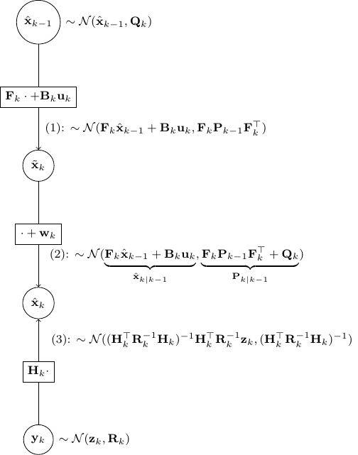
• As shown in the figure above, given and , we have as in (1)

     

  as it is almost identical to Scenario 1 besides a trivial constant shift of .

• Then step (2) is obvious as, is nothing but added by a noise of covariance .
• Now, step (3) is just a direct application of Scenario 2.

Finally, we should combine the estimate from (2) and (3) as independent information using the result in Scenario 3. This gives us the final a posterior estimate of as

Although it is not easy to show immediately, one can verify numerically that the and the mean above are indeed and in the original formulation, respectively.