Category: teaching

This is a rather good read for anyone interested in reproducible research (i.e., everyone who tries to become a researcher as a career)

TLDR:

Why reproducible research

1.  reproducible research helps researchers remember how and why they performed specific analyses during the course of a project.
2.  reproducible research enables researchers to quickly and simply modify analyses and figures.
3.  reproducible research enables quick reconfiguration of previously conducted research.
4.  conducting reproducible research is a strong indicator to fellow researchers of rigor, trustworthiness, and transparency in scientific research.
5.  reproducible research increases paper citation rates (Piwowar et al. 2007, McKiernan et al. 2016) and allows other researchers to cite code and data in addition to publications.

A three-step framework for conducting reproducible research

Before data analysis: data storage and organization

1. data should be backed up at every stage of the research process and stored in multiple locations.
2. Digital data files should be stored in useful, flexible, portable, nonproprietary formats.
3. It is often useful to transform data into a “tidy” format (Wickham 2014) when cleaning up and standardizing raw data.
4. Metadata explaining what was done to clean up the data and what each of the variables means should be stored along with the data.
5. Finally, researchers should organize files in a sensible, user-friendly structure and make sure that all files have informative names.
6. Throughout the research process, from data acquisition to publication, version control can be used to record a project’s history and provide a log of changes that have occurred over the life of a project or research group.

During analysis: best coding practices

1. When possible, all data wrangling and analysis should be performed using coding scripts—as opposed to using interactive or point-and-click tools—so that every step is documented and repeatable by yourself and others.
2. Analytical code should be thoroughly annotated with comments.
3. Following a clean, consistent coding style makes code easier to read.
4. There are several ways to prevent coding mistakes and make code easier to use.
   1. First, researchers should automate repetitive tasks.
   2. Similarly, researchers can use loops to make code more efficient by performing the same task on multiple values or objects in series
   3. A third way to reduce mistakes is to reduce the number of hard-coded values that must be changed to replicate analyses on an updated or new data set.
5.  create a software container, such as a Docker (Merkel 2014) or Singularity (Kurtzer et al. 2017) image (Table 1) for ensuring that analyses can be used in the future

After data analysis: finalizing results and sharing

1. produce tables and figures directly from code than to manipulate these using Adobe Illustrator, Microsoft PowerPoint, or other image editing programs. (comment: for example, can use csvsimple package in latex)
2. make data wrangling, analysis, and creation of figures, tables, and manuscripts a “one-button” process using GNU Make (https://www.gnu.org/software/make/).
3. To increase access to publications, authors can post preprints of final (but preacceptance) versions of manuscripts on a preprint server, or postprints of manuscripts on postprint servers.
4. Data archiving in online general purpose repositories such as Dryad, Zenodo, and Figshare

Useful Links

• Open Science Framework (OSF)
• Singularity
• Docker
• github
• gitlab
• Overleaf
• Rstudio
• Figshare
• Zenodo

Below is a message from Ali Rhoades, an experiential learning coordinator.

 

For students interested in career readiness and job searches, I would encourage them to look into our events page including our Careerapalooza, Career Fair, and other events. Our Careerapalooza is coming up (next Thursday) but this would be a great opportunity for students to informally meet our staff, learn more about our support services (including applying for internship) and join a career community.

Our office just recently launched our Career Communities model, which encourages students to lean into finding internships and jobs specific to their passions and industry, instead of stressing to find experiential learning opportunities strict to their major. For example, if an engineering student was passionate for working in nonprofit, they would find tailored opportunities through their Nonprofit Career Community. This link will also provide them with access to their Handshake accounts (all OU students have free access to this internship and job board) including other helpful resources such as an advisor, additional job posting websites, and career readiness tips. Handshake will be the source where OU posts jobs, internships, externships, co-ops, and fellowships, which has new postings daily. If you would like one of our staff members to visit with your class to share more information about Career Communities and Handshake, please let me know-I’d be happy to set that up for you.

As for micro-internships: OU Career Center will be partnering with Parker Dewey soon, hopefully by the end of September, to have tailored micro-internships exclusively to OU students for local, remote, and regional opportunities that are short term and project based. Until then, students can look for public opportunities through Parker Dewey’s website here.

Define policy and transition probability , the probability of a trajectory equal to

   

Denote the expected return as . Let’s try to find the improve a policy through gradient ascent by updating

   

Policy gradient and REINFORCE

Let’s compute the policy gradient ,

(1)  

With trajectories, we can approximate the gradient as

   

The resulting algorithm is known as REINFORCE.

Actor-critic algorithm

One great thing about the policy-gradient method is that there is much less restriction on the action space than methods like Q-learning. However, one can only learn after a trajectory is finished.  Note that because of causality, reward before the current action should not be affected by the choice of policy. So we can write the policy gradient approximate in REINFORCE instead as

(2)  

Rather than getting the reward from the trajectory directly, an actor-critic algorithm can estimate the return with a critic network . So the policy gradient could be instead approximated by (ignoring discount )

   

Advantage Actor Critic (A2C)

One problem of REINFORCE and the original actor-critic algorithm is high variance. To reduce the variance, we can simply subtract by its average over the action . The difference is known as the advantage function and the resulting is known as the Advantage Actor Critic algorithm. That is the policy gradient will be computed as

   

instead.

 

Reference:

• Deep Reinforcement Learning

Dong has given a very nice talk (slides here) on reinforcement learning (RL) earlier. I learned Q-learning from an online Berkeley lecture several years ago. But I never had a chance to look into SARSA and grasp the concept of on-policy learning before. I think the talk sorted out some of my thoughts.

A background of RL

A typical RL problem involves the interaction between an agent and an environment. The agent will decide on an action based on the current state as it interacts with the environment. Based on this action, the model reaches a new state stochastically with some reward. The agent’s goal is to devise a policy (i.e., determining what action to take under each state) that maximizes the total expected reward. We usually model this setup as the Markov decision process (MDP), where the probability of reaching the next state only depends on the current state and current choice of action (independent of all earlier states) and hence is a Markov model.

Policy and value functions

A policy is just a mapping from each state to an action .  The value function is defined as the expected utility (total reward) of a state given a policy. There are two most common value functions: the state-value function, , which is the expected utility given the current state and policy, and the action-value function, , which is the expected utility given the current action, current state, and policy.

Q-Learning

The main difference of RL from MDP is that the probability is not known in general. If we know this and also the reward for each state, current action, and next state, we can compute the expected utility for any state and appropriate action always. For Q-learning, the goal is precisely to estimate the Q function for the optimal policy by updating Q as

   

where we have to control the degree of exponential smoothing in approximating . When , we do not use exponential smoothing at all.

Note that the equation above only describes how we are going to update , but it does not describe what action should be taken. Of course, we can exploit the estimate of and select the action that maximizes it. However, the early estimates of is bad and so exploiting will work very poorly. Instead, we may simply select the action randomly initially. And as the prediction of improves, exploit the knowledge of and take the action maximizing at times. This is the exploration vs exploitating trade-off. We often denote the probability of exploitation as and we set an algorithm is -greedy when with a probability of that the best action according to the current estimate of is taken.

On policy/Off-policy

In Q-learning, the Q-value is not updated according to data obtained from the actual action that has been taken. There are two terminologies that sometimes confuse me.

• Behavior policy: policy that actually determines the next action
• Target policy: policy that used to evaluate an action and that we are trying to learn

For Q-learning, the behavior policy and target policy apparently are not the same as the action that maximizes does not necessarily be the action that was actually taken.

SARSA

Given an experience (that is why it is called SARSA), we update an estimate of Q instead by

   

It is on-policy as the data used to update (target policy) is directly from the behavior policy that was used to generate the data

Off-policy has the advantage to be more flexible and sample efficient but it could be less stable as well (see [6], for example).

Reference:

• [1] Off Policy vs On Policy Agent Learner – Reinforcement Learning – Machine Learning

• [2] Off-policy vs On-Policy vs Offline Reinforcement Learning Demystified!

• [3] On-Policy v/s Off-Policy Learning

• [4] Off-policy learning

• [5] The False Promise of Off-Policy Reinforcement Learning Algorithms

• [6] Off-policy versus on-policy RL

 

 

 

Here I will derive Kalman filter from belief propagation (BP). While I won’t derive exactly the closed-form expression as Kalman filter, one can verify numerically that the BP procedure below is the same as the standard Kalman filter. For derivation to the exact same expression, please see here.

Kalman filter is a special case of Gaussian BP. It can be easily understood as three different propagation steps as below.

Scenario 1: Passing message from to for

Say , . And as

.

Therefore, .

Scenario 2: Passing message from back to for

This is a bit trickier but still quite simple. Let the covariance of be . And from the perspective of ,

Thus,

Scenario 3: Combining two independent Gaussian messages

Say one message votes for and precision (precision is the inverse of the covariance matrix).  And say another message votes for and precision .

Since

Thus,

BP for Kalman update

Let’s utilize the above to derive the Kalman update rules. We will use almost exactly the same notation as the wiki here. We only replace by and  by to reduce cluttering slightly.

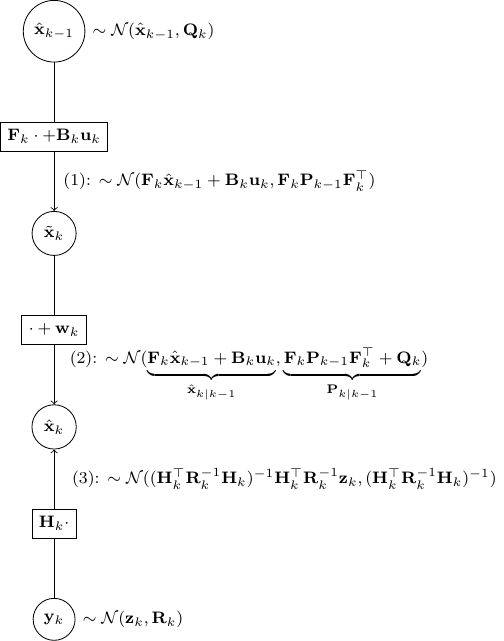
• As shown in the figure above, given and , we have as in (1)

     

  as it is almost identical to Scenario 1 besides a trivial constant shift of .

• Then step (2) is obvious as, is nothing but added by a noise of covariance .
• Now, step (3) is just a direct application of Scenario 2.

Finally, we should combine the estimate from (2) and (3) as independent information using the result in Scenario 3. This gives us the final a posterior estimate of as

   

Although it is not easy to show immediately, one can verify numerically that the and the mean above are indeed and in the original formulation, respectively.

 

Came across two different network architectures that I think can discuss together as I feel that they share a similar core idea. Extract and leverage some global information from the data with global pooling. 

PointNet

The objective of PointNet is to classify each voxel of a point cloud and detect the potential object described by the point cloud. Consequently, each voxel can belong to a different semantic class but they all share the same object class.

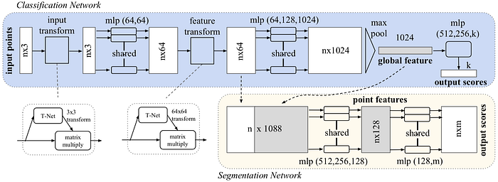
One important property of the point cloud is that all points are not in any particular order. Therefore, it does not make too much sense to train a convolutional layer or fully connected layer to intermix the point. The simplest reasonable operation to combine all information is just pooling (max or average). For PointNet, each point is first individually processed and then a global feature is generated using max pooling. The object described by the point cloud is also classified by the global feature.

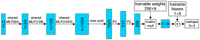
And the input transform and feature transform in the above figure are trainable and will be adapted to the input. This serves the purpose of aligning the point cloud before classification. For example, the T-Net in the input transform is elaborated as shown below.

To classify individual voxel, the global feature is combined with the local feature also generated earlier in the classification network. The combined feature of each voxel will be individually processed into point features, which are then used to classify the semantic class of the voxel.

SENet

SENet was the winner of the classification competition of ImageNet competition in 2017. It reduces the top-5 error rate to 2.251% from the prior 2.991%. The key contribution of SENet is the introduction of the SENet module as follows

The basic idea is very simple. For a feature tensor with $latex C$ channel, we want to adaptively adjust the contribution from each channel through training. Since there is no restriction in the order of the data inside the channel, the most rational thing to summarize that information is simply through pooling. For SE Net module, it is simply done with an average pooling (squeezing). The “squeezed” data are then used to estimate the contribution of each channel (different levels of “excitation”). The computed weights are then used to scale the values of each channel. This SE module can be applied in literally everywhere. For example, it can be combined with inception module to form SE-inception module or ResNet module to form SE-ResNet module as shown below.

Motivation

While Monte Carlo methods have lots of potential applications, we will just name two here as a motivation:

1. Data generation. The generated data can be used for simulation or for visualization purposes.
2. Inference. Infer unknown variables from observations.

For the first application, the use of Monte Carlo is rather straight forward. We will assume the model parameters are known and we can sample parameters sequentially with Gibbs sampling as described below. If all conditional distributions can be sampled directly (more explanation below), we can use regular Monte Carlo without the need for MCMC.

For the second application, there is an additional layer of complication as we typically would like to sample from the posterior distribution for efficiency. But often only the likelihood distributions are specified. In that case, we will need to sample from a proposal distribution and MCMC is needed.

Basic Idea of Monte Carlo Methods

Ultimately, almost all Monte Carlo Methods are doing nothing but estimating the expectation of some function with by

,

where the above is guaranteed by the law of large number for sufficiently large .

For example, in the coin-flipping examples in Q1 of HW5, we can estimate the ultimate probability of head by conducting the Monte Carlo experiment and counting the number of head. More precisely, denote as an indicator function where is 1 when is head. Then

.

The key question here is how we are going to collect samples of , . In this coin-flipping setup, the Monte-Carlo simulation is trivial. We can conduct the experiment exactly as in a real setup. That is, first draw a coin from the jar; that corresponds to sample a binary random variable with the specified probability of getting coins or . Then, based on the outcome of (i.e., which coin that actually picked), we will draw another binary random variable for each coin flip according to the probability of head of the chosen coin.

In the coin-flipping problem, since we are just drawing binary random variables, we can sample the distribution directly without any issue. But for many continuous distributions except a few special cases, direct sampling them is not possible and more involved sampling techniques are needed as described in the following.

This sequential sampling conditioned on previously specified random variables is generally known as Gibbs sampling. Strictly speaking, it is a form of MCMC as we will show later on. But I think it is more appropriate NOT to consider this simple case as MCMC because there is no convergence issue here as you will see that is generally not the case for MCMC.

Basic Sampling Methods

The key question left is how we can sample data from a distribution. For some standard distributions like Gaussian distribution, we can draw samples directly with some well-developed packages. However, there is no direct way of drawing samples for many regular distributions, not to mention those that do not even have a standard form. There are ways to sample any arbitrary distributions, we will mention a couple of simple ones here.

Rejection Sampling

Probably the simplest sampling method is the rejection sampling. Consider drawing sample . Select any “sampleable” distribution such that with some constant . Now, instead of drawing sample from , we will draw from instead. However, in order to have the sample appear to have the same distribution of , we will only keep a fraction of whenever is drawn and discard the rest. To do this, we simply sample a from uniformly after each sampled. And keep the current only if .

Note that in Q4 of HW5, we are essentially doing some form of rejection sampling. Draw the samples from the prior and the likelihood distributions, and then only accept samples that fit the observations. Rejection sampling is simple but it can be quite inefficient. For example, if the current estimates of variables used in sampling are far from the actual values, the sampled outcome most likely will not match well with the observations and we have to reject lots of samples. That’s why other sampling techniques are needed.

Importance Sampling

Rejection sampling is generally very inefficient as a large number of samples can be discarded. If we only care about computing the expection of some function, then we may not need to discard any sample but adjust the weight of each sample instead. Note that

.

Thus, we can estimate the expectation by drawing samples from and compute weighted average of instead. And the corresponding weights are .

Even though we can now utilize all samples, importance sampling has two concerns.

1. Unlike rejection sampling, we do not directly draw samples with the desired distribution. So we can use those samples to do other things rather than computing expectations.
2. The variance of the estimate can be highly sensitive with the choice of . In particular, since the variance of the estimate is , the variance will be especially large if a more probable region in is not covered well by , i.e., we have extensive region where large but .

Markov Chain Monte Carlo

Instead of sampling from directly, Markov chain Monte Carlo (MCMC) methods try to sample from a Markov chain (essentially a probabilistic state model). Probably the two most important properties of the Markov chain are irreducible and aperiodic. We say a Markov chain is irreducible if we can reach any single state to any other state. And we say a Markov chain is periodic if there exist two states such that one state can reach the other state only in a multiple of steps with . If a Markov chain is not periodic, we say it is aperiodic. Under the above two conditions (aperiodic and irreducible), regardless of the initial state, the distribution of states will converge to the steady-state probability distribution asymptotically as time goes to infinity.

Consider any two connected states with transition probabilities (from to ) and (from to ). We say the detailed balance equations are satisfied if . Note that if detailed balance are satisfied among all states, has to be the steady state probability of state . Because the probability “flux” going out from to is exactly canceled by the “flux” coming in from to when the chain reaches this equalibrium.

With the discussion above, we see that one can sample if we can create a Markov chain with designed to be the steady-state probability of the chain (by making sure that detailed balance is satisfied). Note that, however, we have to let the chain to run for a while before the probability distribution converges to the steady-state probability. Thus, samples before the chain reaching equilibrium are discarded. This initial step is known as the “burn-in”. Moreover, since adjacent samples drawn from the chain (even after burn-in) are highly correlated, we may also skip every several samples to reduced correlation.

Metropolis-Hastings

The most well-known MCMC method is the Metropolis-Hastings algorithm. Just as the discussion above, given the distribution , we want to design Markov chain such that satisfies the detailed balance for all states . Given the current state , the immediate question is to which state we should transit to. Assuming that , a simple possibility is just to do a random walk. Essentially perturb with a zero-mean Gaussian random noise. The problem is that the transition probability and the “reverse” transition probability most likely will not satisfy the detailed balance equation . Without loss of generality, we may have . To “balance” the equation, we may reject some of the transition to reduce the probability “flow” on the left hand side. More precisely, let’s denote . Now, we will randomly reject of the transition by drawing a uniform and only allowing transition if .  And similar adjustment is applied to all transitions (including to ). This way, the transition probability from reduces to and so the detailed balance equation is satisfied.

When the transition probabilities from to and from to are equal (i.e., ), note that just simplifies to .

Gibbs Sampling

When the state can be split into multiple component, say . We can transit one component at a time while keeping the rest fixed. For example, we can transit from to with probability . After updating one component, we can update another component in a similar manner until all components are updated. Then, the same procedure can be repeated starting with . As we continue to update the state, the sample drawn will again converge to as the Markov chain reaches equilibrium. This sampling method is known as the Gibbs sampling and can be shown as a special case of Metropolis-Hastings sampling as follows.

Consider the step when transiting from to while keeping the rest of components fixed. as defined earlier is . Thus, Gibbs sampling is really Metropolis-Hasting sampling but with all transitions always be accepted.

Hamiltonian Monte Carlo (HMC)

The trajectory sampled by the Metropolis-Hasting method is essentially a random walk like a drunk man. But we have the complete information of and we know how it looks like. Why don’t we leverage the “geometrical” information of ?

Power of Physics

We definitely can. And recall the Boltzmann distribution (ignoring temperature here) from statistical physics and we can model any distribution with a Boltzmann distribution with appropriate energy function . Further, we expect lower energy states are more likely to happen than higher energy states as expected.

If we think of as the potential energy, a “particle” naturally moves towards lower energy state and the excessive energy will convert to kinetic energy as we learn in Newtonian mechanics. Let’s write the total energy as , where the potential energy is just here. (Sorry for the overloading of symbol here, is commonly used to represent momentum in physics and so we are sticking to that convention here. Please don’t be confuse with the in .) And the kinetic energy with and being the momentum and the mass, respectively. The total energy, , also known as the Hamiltonian is supposed to be conserved as and naturally vary in the phase space . Therefore, .

As we know from classical mechanics, and . For example, let’s consider an object just moving vertically and is the height of the object, then , where is the gravitational force constant.  Then with being the gravitational force and as desired. Moreover, the total energy indeed conserves as and changes as .

Back to Monte Carlo

Why are we talking all these? Because we can draw samples following natural physical trajectories more efficiently than random walks as in Metropolis-Hastings. Given the distribution of interest , we again define the Hamiltonian . Now, instead of trying to draw samples of , we will draw samples of instead. And . So if we marginalize out the momentum , we get back as desired.

And as we samples from the phase space , rather than random walking in the phase space, we can just follow the flow according to Hamiltonian mechanics as described earlier. For example, as we  start from , we may simulate a short time instace to with and . One can also update first and then update . The latter has many different forms and sometimes known as the leapfrog integration. As we apply multiple () leapfrog steps and reach , we may decide whether to accept the sample as in Metropolis-Hasting by evaluating as the transition probabilities are assumed to be the same for both forward and reverse directions. Moreover, if the leapfrog integration is perfect, is supposed to the same as because of conservation of energy. So we have a high chance of accepting a sample.

No-U-Turn Sampling (NUTS)

The main challenge of applying HMC is that the algorithm is quite sensitive to the number of leapfrog step and the step size (more commonly known as ). The goal of NUTS is to automatically select the above two parameters. The main idea is to simulate both forward and backward directions until the algorithm detects reaching a “boundary” and needed to go U-turn. By detecting U-turns, the algorithm can adjust the parameters accordingly. The criterion is simply to check if the momentum starts to turn direction, i.e., or , where and are the two extremes as we go forward and backward in time.

Reference:

1. https://en.wikipedia.org/wiki/Hamiltonian_Monte_Carlo
2. Mackay, Information Theory, Inference, and Learning Algorithms
3. Pattern Recognition and Machine Learning by Bishop
4. A Conceptual Introduction to Hamiltonian Monte Carlo by Michael Betancourt
5. The No-U-Turn Sampler: Adaptively Setting Path Lengths in Hamiltonian Monte Carlo by Matthew D. Hoffman, Andrew Gelman

The three most common graphical models are Bayesian networks (aka directed acyclic graphs), Markov random fields (aka undirected graphs), and factor graphs.

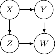
Bayesian networks

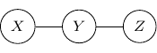
A Bayesian network describes the dependency of variables directly represented by the expansion of the conditional probabilities. Take a very simple example with three variables , and . If the joint distribution can be represented by . Then, the corresponding Bayesian network will be a three-node graph with , and as vertices. And we have two directed edges one from to and another one from to .

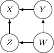
Note that by Bayes rule, the joint probability can be rewritten as . So the following Bayesian network with directed edges one from to and another one from to is identical to the earlier one.

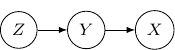
Given , and , we may also have an empty graph with no edge at all. This corresponds to the case when that all three variables are independent as shown below.

We may also have just one edge from to . This corresponds to the case when , which describes the situation when is independent of and as shown below.

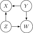
Now, back to the cases with two edges, the ones with two directed edges flowing the same direction will just have the same structure as the example we have earlier. So let’s look at other interesting setups. First, let’s consider the case that both directed edges are coming out of the same variable. For example, we have two directed edges from to and from to as shown below.

This corresponds to the joint distribution . So this case is actually the same as the case we have earlier after all. Note that however, this equivalence is not generalizable when we have more variables. For example, say we also have another variable and an edge from to .

And if we have the direction of the edge to flipped as below, and become independent but the earlier representation does not imply that.

Now, let’s remove and assume we only have three variables and two edges as described earlier. For all cases we have above (say edges from to and to ), the variables at the two ends and are not independent. But they are independent given the variable in the middle. Be very careful since the situation will be totally flipped as we change the direction of the edge from to in the following.

The corresponding joint probability for the above graph is . We have and are independent as . On the other hand, we don’t have . And so and are not conditional independent given is observed. The classic example is and are two independent binary outcome taking values and , where is the xor operation such that and . As the xor equation also implies , is completely determined by when is given. Therefore, is in no way to be independent of given . Quite the opposite, and are maximally correlated given .

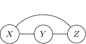
Let’s consider the case with three edges. Note that we can’t have edges forming a loop since Bayesian networks have to be an acyclic graph. A possibility can be having three directed edges one from to , one from to , and the last one from to as shown below.

In this case, the joint probability will be . Note that the joint probability can be directly obtained by Bayes rule and so the graph itself does not assume any dependence/independence structure. The other Bayesian networks with three edges will all be identical and do not imply any independence among variables as well.

As we see above, the dependency of variables can be derived from a Bayesian network as the joint probability of the variables can be written down directly. Actually, an important function of all graphical models is to represent such dependency among variables. In terms of Bayesian networks, there is a fancy term known as d-separation which basically refers to the fact that some variables are conditional independent from another given some other variables as can be observed from the Bayesian network. Rather than trying to memorize the rules of d-separation, I think it is much easier to understand the simple three variables examples and realize under what situations that variables are independent or conditionally independent. And for two variables to be conditionally independent of one another, all potential paths of dependency have to be broken down. For example, for the three variables three edges example above (with edges , , and ), observing will break the dependency path of for and . But they are not yet conditionally independent because of the latter path .

Let’s consider one last example with four variables and , and three edges (, , and ) below.

Note that as root nodes, and are independent. And thus and are independent as well since only depends on . On the other hand, if is observed, and are no longer independent. And thus and are not conditionally independent given .

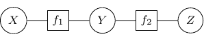
Undirected graphs and factor graphs

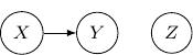
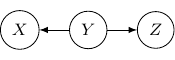
Compared with Bayesian networks, dependency between variables is much easier to understand. Two variables are independent if they are not connected and two variables are conditionally independent given some variables if the variables are not connected if the vertices of the given variables are removed from the graph.

For example, consider a simple undirected graph above with three variables , , and with two edges and . Variables and are then independent given .

By Hammersley-Clifford theorem, the joint probability of any undirected graph models can be represented into the product of factor function of the form . For example, the joint probability of the above graph can be rewritten as with , and . We can use a bipartite graph to represent the factor product above in the following.

1. Represent each factor in the product with a vertex (typically known as factor node and display with a square by convention)
2. Represent each random variable with a vertex (typically known as a variable node)
3. Connect each factor node to all of its argument with an undirected edge

The graph constructed above is known as a factor graph. With the example described above, we have a factor graph as shown below.

The moralization of Bayesian networks

Consider again the simple Bayesian network with variables , , and , and edges and below.

What should be the corresponding undirected graph to represent this structure?

It is tempting to have the simple undirected graph before with edges and below.

However, it does not correctly capture the dependency between and . Recall that when is observed or given, and are no longer independent. But for the undirected graph above, it exactly captured the opposite. That is and are conditionally independent given . So, to ensure that this conditional independence is not artificially augmented into the model, what we need to do is to add an additional edge as shown below.

This procedure is sometimes known as moralization. It came for the analogy of a child born out of wedlock and the parents should get married and “moralized”.

Undirected graphs cannot represent all Bayesian networks

Despite the additional edge , the resulting graph, a fully connected graph with three vertices , , and still does not accurately describe the original Bayesian network. Namely, in the original network, and are independent but the undirected graph does not capture that.

So if either way the model is not a perfect representation, why we bother to moralize the parents anyway? Note that for each edge we added, we reduce the (dependency) assumption behind the model. Solving a relaxed problem with fewer assumptions will not give us the wrong solution. Just maybe will make the problem more difficult to solve. But adding an incorrect assumption that does not exist in the original problem definitely can lead to a very wrong result. So the moralization step is essential when we convert directed to undirected graphs. Make sure you keep all parents in wedlock.

Bayesian networks cannot represent all undirected graphs

Then, does that mean that Bayesian networks are more powerful or have a higher representation power than undirected graphs? Not really also, as there are undirected graphs that cannot be captured by Bayesian networks as well.

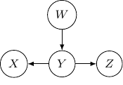
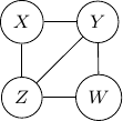
Consider undirected graph with four variables and and four edges , , , and as shown below.

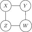
Note that we have conditional independence of and given and . This conditional independence is captured only by one of the following three Bayesian networks.

       

Because of the moralization we discussed earlier, when we convert the above models into undirected graphs, they all require us to add an additional edge between parents and resulting in the undirected graph below.

Note that this undirected graph is definitely not the same as the earlier one since it cannot capture the conditional independence between and given and . In conclusion, no Bayesian network can exactly capture the structure of the square undirected graph above.

Assume that there are two biased coins. Coin A heavily biased towards head with the probability of head equal to 0.9. And Coin B is heavily biased towards tail with the probability of tail equal to 0.9. Now, we randomly and equally likely select one of the coins and toss it twice. Let’s call the outcome and . Now, the question is, what is the mutual information between and ?

I put a similar question as above in a midterm, and I didn’t expect to stumble the entire class.

All students thought that the mutual information because the two outcomes are independent. When we toss a coin sequentially, the outcomes are supposed to be independent, right? Yes, but that is only when we know what coin we are tossing.

Think intuitively with the above example. If we didn’t toss the coin twice, but toss it ten times and got ten heads. What do we expect the outcome to be if we toss it another time?

I think an intelligent guess should be another head. Because given the ten heads we got earlier, it has a very high chance that the picked coin is Coin A. And so the next toss is very likely to be the head as well.

Now, the same argument holds when we are back to the original setup. When the first toss is head, the second toss is likely to be head as well. So and are in no way to be independent.

So what is ?

Let’s compute and .

Denote as the coin that we pick.

So bit.

Now, for , note that

Therefore, bit.

So bit.

Note that this is an example that variables are conditional independent but not independent. More precisely, we have but .

Probability education trap

I wondered a little bit why none of my students could answer the above question. I blame a trap that is embedded in most elementary probability courses. We were always introduced with a consecutive coin tossing or dice throwing example with each subsequent event to be independent of the earlier event. In those examples, we always assume that the probabilities of getting all outcomes are known but this assumption was never emphasized. As we see in the above example, even each subsequent tossing or throwing is independent relative to the current coin or the current dice, overall those events are not independent when the statistics behind the coin and dice are not known.

Actually, this also makes some “pseudo-science” not really that non-scientific after all. For example, we all tend to believe that the gender of a newborn is close to random and hence unpredictable. But what if there is some hidden variable that affects the gender of a newborn. And that factor may have a strong bias towards one gender over another. Then, it probably is not really that unlikely for someone to have five consecutive girls or six consecutive sons. Of course, I also tend to believe that the probability of a newborn to be a boy or a girl is very close to one half. A less extreme example may occur at the casino. If we believe that the odd from each lottery machine in a casino is not so perfectly tune (before the digital age, that is probably much more likely), then there is a chance that some machine has a higher average reward than another one. Then, a gambler trying to select a lottery machine to play is an essential strategy to win and is not really superstition after all. Of course, this is just the multi-armed bandit problem.

Independence and conditional independence are one of the most basic concepts in probabilities. Two random variables are independent, as the term suggested, if the outcome of one variable should not affect the outcome of another. Mathematically, two variables and are independent if

for any outcome for variable and outcome for variable . And we often indicate this independece by .

Let’s inspect this definition more carefully, given and by Bayes’ rule, the probability of is

. Indeed the probability does not depend on the outcome of and so and are independent.

Similarly, when we say and are conditionally independent given , it means that knowing , and become independent. Note that and do not need to be independent to start with. Many students have the misconceptions that independence implies conditional independence, or vice versa. The fact is that they are completely unrelated concepts. We can easily find examples that variables are independent but not conditional independent and vice versa. And also examples that variables are both independent and conditional independent. And of course cases when neither independence is satisfied.

Mathematically, we denote the independence by , and we have

for any , and .

Note that the definition above implies that . Hence, indeed if we are given , the probability of does not dependent on the outcome of . So it depicts well the conditional independence that we anticipated.