Motivation
While Monte Carlo methods have lots of potential applications, we will just name two here as a motivation:
- Data generation. The generated data can be used for simulation or for visualization purposes.
- Inference. Infer unknown variables from observations.
For the first application, the use of Monte Carlo is rather straight forward. We will assume the model parameters are known and we can sample parameters sequentially with Gibbs sampling as described below. If all conditional distributions can be sampled directly (more explanation below), we can use regular Monte Carlo without the need for MCMC.
For the second application, there is an additional layer of complication as we typically would like to sample from the posterior distribution for efficiency. But often only the likelihood distributions are specified. In that case, we will need to sample from a proposal distribution and MCMC is needed.
Basic Idea of Monte Carlo Methods
Ultimately, almost all Monte Carlo Methods are doing nothing but estimating the expectation of some function  with
with  by
by
![E_{X\sim p(x)}[f(X)] \approx \frac{1}{N} \sum_{i=1}^N f(x_i)](https://outliip.org/wp-content/ql-cache/quicklatex.com-5508485a4aa7e8f10804dd37ae794026_l3.png "Rendered by QuickLaTeX.com") ,
,
where the above is guaranteed by the law of large number for sufficiently large  .
.
For example, in the coin-flipping examples in Q1 of HW5, we can estimate the ultimate probability of head by conducting the Monte Carlo experiment and counting the number of head. More precisely, denote  as an indicator function where is 1 when
  is head. Then
![Pr(Y=H)=E_{Y \sim p(y)}[i_H(Y)] \approx \frac{1}{N} \sum_{i=1}^N i_H(y_i)](https://outliip.org/wp-content/ql-cache/quicklatex.com-771f2ed0bbbc8dff794ec970b225b31d_l3.png "Rendered by QuickLaTeX.com") .
.
The key question here is how we are going to collect samples of ,  . In this coin-flipping setup, the Monte-Carlo simulation is trivial. We can conduct the experiment exactly as in a real setup. That is, first draw a coin from the jar; that corresponds to sample a binary random variable
  with the specified probability of getting coins
  or
or  . Then, based on the outcome of (i.e., which coin that actually picked), we will draw another binary random variable for each coin flip according to the probability of head of the chosen coin.
In the coin-flipping problem, since we are just drawing binary random variables, we can sample the distribution directly without any issue. But for many continuous distributions except a few special cases, direct sampling them is not possible and more involved sampling techniques are needed as described in the following.
This sequential sampling conditioned on previously specified random variables is generally known as Gibbs sampling. Strictly speaking, it is a form of MCMC as we will show later on. But I think it is more appropriate NOT to consider this simple case as MCMC because there is no convergence issue here as you will see that is generally not the case for MCMC.
Basic Sampling Methods
The key question left is how we can sample data from a distribution. For some standard distributions like Gaussian distribution, we can draw samples directly with some well-developed packages. However, there is no direct way of drawing samples for many regular distributions, not to mention those that do not even have a standard form. There are ways to sample any arbitrary distributions, we will mention a couple of simple ones here.
Rejection Sampling
Probably the simplest sampling method is the rejection sampling. Consider drawing sample . Select any “sampleable” distribution  such that
  with some constant
  . Now, instead of drawing sample from
  , we will draw from instead. However, in order to have the sample appear to have the same distribution of , we will only keep a fraction
  of
of  whenever is drawn and discard the rest. To do this, we simply sample a
  from
from ![[0,1]](https://outliip.org/wp-content/ql-cache/quicklatex.com-25b6d943ab489c05a3dbd5ea29087a48_l3.png "Rendered by QuickLaTeX.com") uniformly after each
uniformly after each  sampled. And keep the current only if
  .
.
Note that in Q4 of HW5, we are essentially doing some form of rejection sampling. Draw the samples from the prior and the likelihood distributions, and then only accept samples that fit the observations. Rejection sampling is simple but it can be quite inefficient. For example, if the current estimates of variables used in sampling are far from the actual values, the sampled outcome most likely will not match well with the observations and we have to reject lots of samples. That’s why other sampling techniques are needed.
Importance Sampling
Rejection sampling is generally very inefficient as a large number of samples can be discarded. If we only care about computing the expection of some function, then we may not need to discard any sample but adjust the weight of each sample instead. Note that
![E_{X\sim p(x)}[f(X)]=\int f(x) p(x) dx = \int \left[f(x)\frac{p(x)}{q(x)}\right] q(x) dx= E_{X\sim q(x)}\left[f(X)\frac{p(X)}{q(X)}\right]](https://outliip.org/wp-content/ql-cache/quicklatex.com-d44ddc9ce7e912f6d9872ce5cced50c1_l3.png "Rendered by QuickLaTeX.com") .
.
Thus, we can estimate the expectation by drawing samples from and compute weighted average of instead. And the corresponding weights are  .
.
Even though we can now utilize all samples, importance sampling has two concerns.
- Unlike rejection sampling, we do not directly draw samples with the desired distribution. So we can use those samples to do other things rather than computing expectations.
- The variance of the estimate can be highly sensitive with the choice of
 . In particular, since the variance of the estimate is
 ![\frac{1}{N}E\left[ f(X)\frac{p(X)}{q(X)}\right]](https://outliip.org/wp-content/ql-cache/quicklatex.com-8dbe52483531c01ca6f87a0182b0ba52_l3.png "Rendered by QuickLaTeX.com") , the variance will be especially large if a more probable region in is not covered well by , i.e., we have extensive region where large but
, the variance will be especially large if a more probable region in is not covered well by , i.e., we have extensive region where large but  .
.
Markov Chain Monte Carlo
Instead of sampling from directly, Markov chain Monte Carlo (MCMC) methods try to sample from a Markov chain (essentially a probabilistic state model). Probably the two most important properties of the Markov chain are irreducible and aperiodic. We say a Markov chain is irreducible if we can reach any single state to any other state. And we say a Markov chain is periodic if there exist two states such that one state can reach the other state only in a multiple of  steps with
  . If a Markov chain is not periodic, we say it is aperiodic. Under the above two conditions (aperiodic and irreducible), regardless of the initial state, the distribution of states will converge to the steady-state probability distribution asymptotically as time goes to infinity.
Consider any two connected states with transition probabilities  (from to ) and
  (from to ). We say the detailed balance equations are satisfied if
  . Note that if detailed balance are satisfied among all states, has to be the steady state probability of state . Because the probability “flux” going out from to is exactly canceled by the “flux” coming in from to when the chain reaches this equalibrium.
With the discussion above, we see that one can sample if we can create a Markov chain with designed to be the steady-state probability of the chain (by making sure that detailed balance is satisfied). Note that, however, we have to let the chain to run for a while before the probability distribution converges to the steady-state probability. Thus, samples before the chain reaching equilibrium are discarded. This initial step is known as the “burn-in”. Moreover, since adjacent samples drawn from the chain (even after burn-in) are highly correlated, we may also skip every several samples to reduced correlation.
Metropolis-Hastings
The most well-known MCMC method is the Metropolis-Hastings algorithm. Just as the discussion above, given the distribution , we want to design Markov chain such that satisfies the detailed balance for all states . Given the current state , the immediate question is to which state we should transit to. Assuming that  , a simple possibility is just to do a random walk. Essentially perturb with a zero-mean Gaussian random noise. The problem is that the transition probability
  and the “reverse” transition probability
  most likely will not satisfy the detailed balance equation
  . Without loss of generality, we may have
  . To “balance” the equation, we may reject some of the transition to reduce the probability “flow” on the left hand side. More precisely, let’s denote
  . Now, we will randomly reject
  of the transition by drawing a uniform
 ![Z\in [0,1]](https://outliip.org/wp-content/ql-cache/quicklatex.com-24589ead3a6cd5416c8d4342cdc5f35c_l3.png "Rendered by QuickLaTeX.com") and only allowing transition if
and only allowing transition if  . And similar adjustment is applied to all transitions (including to ). This way, the transition probability from reduces to
  and so the detailed balance equation is satisfied.
When the transition probabilities from to and from to are equal (i.e.,  ), note that just simplifies to
  .
.
Gibbs Sampling
When the state can be split into multiple component, say  . We can transit one component at a time while keeping the rest fixed. For example, we can transit from
  to
to  with probability
  . After updating one component, we can update another component in a similar manner until all components are updated. Then, the same procedure can be repeated starting with . As we continue to update the state, the sample drawn will again converge to as the Markov chain reaches equilibrium. This sampling method is known as the Gibbs sampling and can be shown as a special case of Metropolis-Hastings sampling as follows.
Consider the step when transiting from to while keeping the rest of components fixed.  as defined earlier is
  . Thus, Gibbs sampling is really Metropolis-Hasting sampling but with all transitions always be accepted.
Hamiltonian Monte Carlo (HMC)
The trajectory sampled by the Metropolis-Hasting method is essentially a random walk like a drunk man. But we have the complete information of and we know how it looks like. Why don’t we leverage the “geometrical” information of ?
Power of Physics
We definitely can. And recall the Boltzmann distribution  (ignoring temperature here) from statistical physics and we can model any distribution with a Boltzmann distribution with appropriate energy function
  . Further, we expect lower energy states are more likely to happen than higher energy states as expected.
If we think of  as the potential energy, a “particle” naturally moves towards lower energy state and the excessive energy will convert to kinetic energy as we learn in Newtonian mechanics. Let’s write the total energy as
  , where the potential energy
  is just here. (Sorry for the overloading of symbol
  here, is commonly used to represent momentum in physics and so we are sticking to that convention here. Please don’t be confuse with the in .) And the kinetic energy
  with and
  being the momentum and the mass, respectively. The total energy,
  , also known as the Hamiltonian is supposed to be conserved as and naturally vary in the phase space
  . Therefore,
  .
.
As we know from classical mechanics,  and
and  . For example, let’s consider an object just moving vertically and is the height of the object, then
  , where
  is the gravitational force constant. Then
  with
with  being the gravitational force and
  as desired. Moreover, the total energy indeed conserves as and
  changes as
  .
.
Back to Monte Carlo
Why are we talking all these? Because we can draw samples following natural physical trajectories more efficiently than random walks as in Metropolis-Hastings. Given the distribution of interest , we again define the Hamiltonian  . Now, instead of trying to draw samples of , we will draw samples of instead. And
  . So if we marginalize out the momentum , we get back as desired.
And as we samples from the phase space , rather than random walking in the phase space, we can just follow the flow according to Hamiltonian mechanics as described earlier. For example, as we start from , we may simulate a short time instace  to
to  with
with  and
and  . One can also update first and then update . The latter has many different forms and sometimes known as the leapfrog integration. As we apply multiple (
 ) leapfrog steps and reach
  , we may decide whether to accept the sample as in Metropolis-Hasting by evaluating
  as the transition probabilities are assumed to be the same for both forward and reverse directions. Moreover, if the leapfrog integration is perfect, is supposed to the same as
  because of conservation of energy. So we have a high chance of accepting a sample.
No-U-Turn Sampling (NUTS)
The main challenge of applying HMC is that the algorithm is quite sensitive to the number of leapfrog step and the step size (more commonly known as  ). The goal of NUTS is to automatically select the above two parameters. The main idea is to simulate both forward and backward directions until the algorithm detects reaching a “boundary” and needed to go U-turn. By detecting U-turns, the algorithm can adjust the parameters accordingly. The criterion is simply to check if the momentum starts to turn direction, i.e.,
  or
or  , where
  and
and  are the two extremes as we go forward and backward in time.
Reference:
- https://en.wikipedia.org/wiki/Hamiltonian_Monte_Carlo
- Mackay, Information Theory, Inference, and Learning Algorithms
- Pattern Recognition and Machine Learning by Bishop
- A Conceptual Introduction to Hamiltonian Monte Carlo
 by Michael Betancourt
- The No-U-Turn Sampler: Adaptively Setting Path Lengths in Hamiltonian Monte Carlo by Matthew D. Hoffman, Andrew Gelman


 , and
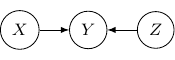
, and  . Then, the corresponding Bayesian network will be a three-node graph with
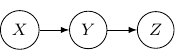
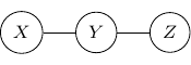
 . So the following Bayesian network with directed edges one from
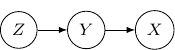
 that all three variables are independent as shown below.
 . This corresponds to the case when
  , which describes the situation when
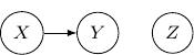
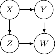
 . So this case is actually the same as the case we have earlier after all. Note that however, this equivalence is not generalizable when we have more variables. For example, say we also have another variable
  and an edge from
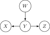
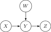
 . We have
  . On the other hand, we don’t have
  . And so
  and
and  , where
  is the xor operation such that
  and
and  . As the xor equation also implies
  ,
, 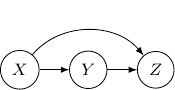
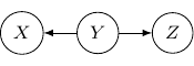
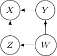
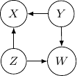
 . Note that the joint probability can be directly obtained by Bayes rule and so the graph itself does not assume any dependence/independence structure. The other Bayesian networks with three edges will all be identical and do not imply any independence among variables as well.
 ,
,  , and
, and  ), observing
  for
for  and
and  , and
, and  ) below.
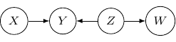
 and
and  . Variables
  . For example, the joint probability of the above graph can be rewritten as
  with
with  , and
, and  . We can use a bipartite graph to represent the factor product above in the following.
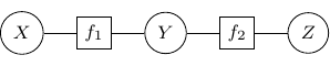
 as shown below.
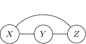
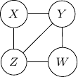
 , the resulting graph, a fully connected graph with three vertices
  and
and  ,
,  ,
,  , and
, and  as shown below.
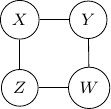
 and
and  . Now, the question is, what is the mutual information between
  because the two outcomes are independent. When we toss a coin sequentially, the outcomes are supposed to be independent, right? Yes, but that is only when we know what coin we are tossing.
 ?
?
 and
and  .
.
 bit.
bit.


![H(Y_1,Y_2)=H([0.41,0.41,0.09,0.09])=1.68](https://outliip.org/wp-content/ql-cache/quicklatex.com-666d39ab22bd22c580a5f2b87072b995_l3.png "Rendered by QuickLaTeX.com") bit.
bit. bit.
bit. but
but  .
. for any outcome
  .
. and by Bayes’ rule, the probability of
  is
is . Indeed the probability does not depend on the outcome of
  , and we have
 for any
  , and
, and  .
. . Hence, indeed if we are given