Here I will derive Kalman filter from belief propagation (BP). While I won’t derive exactly the closed-form expression as Kalman filter, one can verify numerically that the BP procedure below is the same as the standard Kalman filter. For derivation to the exact same expression, please see here.
Kalman filter is a special case of Gaussian BP. It can be easily understood as three different propagation steps as below.
Scenario 1: Passing message from  to
to  for
for 
Say  ,
, ![E[Y] = E[AX] = A\mu_X](https://outliip.org/wp-content/ql-cache/quicklatex.com-c54020001728bf856783511520581ed8_l3.png "Rendered by QuickLaTeX.com") . And as
. And as
![\Sigma_Y=E[(Y-\mu_Y)(Y-\mu_Y)^\top]=E[(AX-A\mu_X)(AX - A\mu_X)^\top]](https://outliip.org/wp-content/ql-cache/quicklatex.com-a79f618ab50f04e839d9fdcd4595b805_l3.png "Rendered by QuickLaTeX.com")
![=E[A(X-\mu_X)(X-\mu_X)^\top A^\top]=A\Sigma_X A^\top](https://outliip.org/wp-content/ql-cache/quicklatex.com-eb07da3da8d39ef06f2211eade38cb34_l3.png "Rendered by QuickLaTeX.com") .
.
Therefore,  .
.
Scenario 2: Passing message from back to for
This is a bit trickier but still quite simple. Let the covariance of be  . And from the perspective of ,


Thus, 
Scenario 3: Combining two independent Gaussian messages
Say one message votes for  and precision
  (precision is the inverse of the covariance matrix). And say another message votes for
  and precision
  .
.
Since


Thus, 
BP for Kalman update
Let’s utilize the above to derive the Kalman update rules. We will use almost exactly the same notation as the wiki here. We only replace  by
by  and
and  by
by  to reduce cluttering slightly.
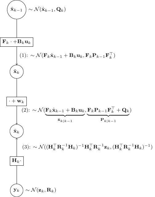
- As shown in the figure above, given
 and
and  , we have as in (1)
![\[\tilde{\bf x}_k \sim \mathcal{N}({\bf F}_k \hat{\bf x}_{k-1} + {\bf B}_k {\bf u}_k, {\bf F}_k {\bf P}_{k-1}{\bf F}_k^\top)\]](https://outliip.org/wp-content/ql-cache/quicklatex.com-53c4647000975eab4573bbd27baa466c_l3.png "Rendered by QuickLaTeX.com")
as it is almost identical to Scenario 1 besides a trivial constant shift of
 .
. - Then step (2) is obvious as,
 is nothing but
  added by a noise of covariance
  .
. - Now, step (3) is just a direct application of Scenario 2.
Finally, we should combine the estimate from (2) and (3) as independent information using the result in Scenario 3. This gives us the final a posterior estimate of  as
as
![\[\mathcal{N}\left(\Sigma({\bf P}_{k|k-1}^{-1} \hat{\bf x}_{k|k-1} +{\bf H}_k^\top {\bf R}_k^{-1} {\bf z}_k),\underset{\Sigma}{\underbrace{({\bf P}^{-1}_{k|k-1}+{\bf H}^\top_k {\bf R}^{-1}_k {\bf H}_k)^{-1}}}\right)\]](https://outliip.org/wp-content/ql-cache/quicklatex.com-f728e11ea7c6193a812c8c9305dcdd48_l3.png "Rendered by QuickLaTeX.com")
Although it is not easy to show immediately, one can verify numerically that the  and the mean above are indeed
  and
and  in the original formulation, respectively.