Bayesian networks, Markov random fields, and factor graphs

The three most common graphical models are Bayesian networks (aka directed acyclic graphs), Markov random fields (aka undirected graphs), and factor graphs.

Bayesian networks

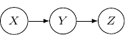
A Bayesian network describes the dependency of variables directly represented by the expansion of the conditional probabilities. Take a very simple example with three variables $X, Y$ , and $Z$ . If the joint distribution can be represented by $p(x) p(y|x) p(z|y)$ . Then, the corresponding Bayesian network will be a three-node graph with $X, Y$ , and $Z$ as vertices. And we have two directed edges one from $X$ to $Y$ and another one from $Y$ to $Z$ .

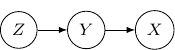
Note that by Bayes rule, the joint probability can be rewritten as $p(z) p(y|z) p(x|y)$ . So the following Bayesian network with directed edges one from $Z$ to $Y$ and another one from $Y$ to $X$ is identical to the earlier one.

Given $X, Y$ , and $Z$ , we may also have an empty graph with no edge at all. This corresponds to the case when $p(x,y,z)=p(x)p(y)p(z)$ that all three variables are independent as shown below.

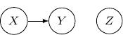
We may also have just one edge from $x$ to $y$ . This corresponds to the case when $p(x,y,z)=p(x)p(y|x) p(z)$ , which describes the situation when $Z$ is independent of $X$ and $Y$ as shown below.

Now, back to the cases with two edges, the ones with two directed edges flowing the same direction will just have the same structure as the example we have earlier. So let’s look at other interesting setups. First, let’s consider the case that both directed edges are coming out of the same variable. For example, we have two directed edges from $Y$ to $X$ and from $Y$ to $Z$ as shown below.

This corresponds to the joint distribution $p(x,y,z)=p(y)p(x|y)p(z|y)=p(x)p(y|x)p(z|y)$ . So this case is actually the same as the case we have earlier after all. Note that however, this equivalence is not generalizable when we have more variables. For example, say we also have another variable $W$ and an edge from $W$ to $Y$ .

And if we have the direction of the edge $Y$ to $X$ flipped as below, $W$ and $X$ become independent but the earlier representation does not imply that.

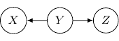
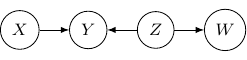
Now, let’s remove $W$ and assume we only have three variables and two edges as described earlier. For all cases we have above (say edges from $X$ to $Y$ and $Y$ to $Z$ ), the variables at the two ends $X$ and $Z$ are not independent. But they are independent given the variable $Y$ in the middle. Be very careful since the situation will be totally flipped as we change the direction of the edge from $Y$ to $Z$ in the following.

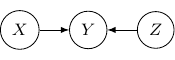
The corresponding joint probability for the above graph is $p(x,y,z)=p(x) p(z) p(y|x,z)$ . We have $X$ and $Z$ are independent as $p(x,z)=\sum_z p(x,y,z)=\sum_z p(x)p(z)p(y|x,z)=p(x)p(z)$ . On the other hand, we don’t have $p(x,z|y)=p(x|y)p(z|y)$ . And so $X$ and $Z$ are not conditional independent given $Y$ is observed. The classic example is $X$ and $Z$ are two independent binary outcome taking values $\{0,1\}$ and $Y = X \oplus Z$ , where $\oplus$ is the xor operation such that $1\oplus 1=0\oplus 0=0$ and $0\oplus 1=1 \oplus 0=1$ . As the xor equation also implies $X =Z \oplus Y$ , $X$ is completely determined by $Z$ when $Y$ is given. Therefore, $X$ is in no way to be independent of $Z$ given $Y$ . Quite the opposite, $X$ and $Z$ are maximally correlated given $Y$ .

Let’s consider the case with three edges. Note that we can’t have edges forming a loop since Bayesian networks have to be an acyclic graph. A possibility can be having three directed edges one from $X$ to $Y$ , one from $Y$ to $Z$ , and the last one from $X$ to $Z$ as shown below.

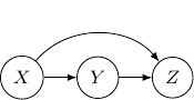
In this case, the joint probability will be $p(x,y,z)=p(x)p(y|x)p(z|x,y)$ . Note that the joint probability can be directly obtained by Bayes rule and so the graph itself does not assume any dependence/independence structure. The other Bayesian networks with three edges will all be identical and do not imply any independence among variables as well.

As we see above, the dependency of variables can be derived from a Bayesian network as the joint probability of the variables can be written down directly. Actually, an important function of all graphical models is to represent such dependency among variables. In terms of Bayesian networks, there is a fancy term known as d-separation which basically refers to the fact that some variables are conditional independent from another given some other variables as can be observed from the Bayesian network. Rather than trying to memorize the rules of d-separation, I think it is much easier to understand the simple three variables examples and realize under what situations that variables are independent or conditionally independent. And for two variables to be conditionally independent of one another, all potential paths of dependency have to be broken down. For example, for the three variables three edges example above (with edges $X\rightarrow Y$ , $Y\rightarrow Z$ , and $X\rightarrow Z$ ), observing $Y$ will break the dependency path of $X\rightarrow Y\rightarrow Z$ for $X$ and $Z$ . But they are not yet conditionally independent because of the latter path $X\rightarrow Z$ .

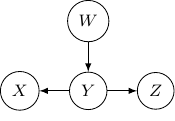
Let’s consider one last example with four variables $X,Y,Z$ and $W$ , and three edges ( $X\rightarrow Y$ , $Z\rightarrow Y$ , and $Z\rightarrow W$ ) below.

Note that as root nodes, $X$ and $Z$ are independent. And thus $X$ and $W$ are independent as well since $W$ only depends on $Z$ . On the other hand, if $Y$ is observed, $X$ and $Z$ are no longer independent. And thus $X$ and $W$ are not conditionally independent given $Y$ .

Undirected graphs and factor graphs

Compared with Bayesian networks, dependency between variables is much easier to understand. Two variables are independent if they are not connected and two variables are conditionally independent given some variables if the variables are not connected if the vertices of the given variables are removed from the graph.

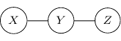
For example, consider a simple undirected graph above with three variables $X$ , $Y$ , and $Z$ with two edges $X - Y$ and $Y-Z$ . Variables $X$ and $Z$ are then independent given $Y$ .

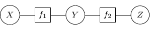
By Hammersley-Clifford theorem, the joint probability of any undirected graph models can be represented into the product of factor function of the form $\prod_{\bf i} \phi_i ({\bf x}_i)$ . For example, the joint probability of the above graph can be rewritten as $f_1(x,y)f_2(y,z)$ with $f_1(x,y)=p(x|y)$ , and $f_2(y,z)=p(y)p(z|y)$ . We can use a bipartite graph to represent the factor product above in the following.

Represent each factor in the product with a vertex (typically known as factor node and display with a square by convention)
Represent each random variable with a vertex (typically known as a variable node)
Connect each factor node to all of its argument with an undirected edge

The graph constructed above is known as a factor graph. With the example described above, we have a factor graph as shown below.

The moralization of Bayesian networks

Consider again the simple Bayesian network with variables $X$ , $Y$ , and $Z$ , and edges $X\rightarrow Y$ and $Z\rightarrow Y$ below.

What should be the corresponding undirected graph to represent this structure?

It is tempting to have the simple undirected graph before with edges $X - Y$ and $Y-Z$ below.

However, it does not correctly capture the dependency between $X$ and $Z$ . Recall that when $Y$ is observed or given, $X$ and $Z$ are no longer independent. But for the undirected graph above, it exactly captured the opposite. That is $X$ and $Z$ are conditionally independent given $Y$ . So, to ensure that this conditional independence is not artificially augmented into the model, what we need to do is to add an additional edge $X - Z$ as shown below.

This procedure is sometimes known as moralization. It came for the analogy of a child born out of wedlock and the parents should get married and “moralized”.

Undirected graphs cannot represent all Bayesian networks

Despite the additional edge $X-Z$ , the resulting graph, a fully connected graph with three vertices $X$ , $Y$ , and $Z$ still does not accurately describe the original Bayesian network. Namely, in the original network, $X$ and $Z$ are independent but the undirected graph does not capture that.

So if either way the model is not a perfect representation, why we bother to moralize the parents anyway? Note that for each edge we added, we reduce the (dependency) assumption behind the model. Solving a relaxed problem with fewer assumptions will not give us the wrong solution. Just maybe will make the problem more difficult to solve. But adding an incorrect assumption that does not exist in the original problem definitely can lead to a very wrong result. So the moralization step is essential when we convert directed to undirected graphs. Make sure you keep all parents in wedlock.

Bayesian networks cannot represent all undirected graphs

Then, does that mean that Bayesian networks are more powerful or have a higher representation power than undirected graphs? Not really also, as there are undirected graphs that cannot be captured by Bayesian networks as well.

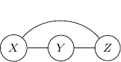
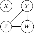
Consider undirected graph with four variables $X, Y, Z,$ and $W$ and four edges $X-Y$ , $Y-W$ , $Z-W$ , and $Z-X$ as shown below.

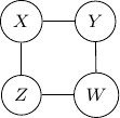
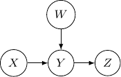
Note that we have conditional independence of $X$ and $W$ given $Y$ and $Z$ . This conditional independence is captured only by one of the following three Bayesian networks.

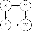
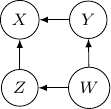
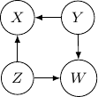
Because of the moralization we discussed earlier, when we convert the above models into undirected graphs, they all require us to add an additional edge between parents $Y$ and $Z$ resulting in the undirected graph below.

Note that this undirected graph is definitely not the same as the earlier one since it cannot capture the conditional independence between $Y$ and $Z$ given $W$ and $X$ . In conclusion, no Bayesian network can exactly capture the structure of the square undirected graph above.

M	T	W	T	F	S	S
						1
2	3	4	5	6	7	8
9	10	11	12	13	14	15
16	17	18	19	20	21	22
23	24	25	26	27	28	29
30